The Bootstrap
Introduction
The bootstrap is a method for estimating parameters and confidence
intervals. It makes few assumptions about the data and is therefore
useful even when conventional statistical methods are inappropriate.
In addition, it is remarkably flexible: you can use it to estimate
essentially anything.
Let us start with an example. Consider the median of a sample of size
N, drawn at random from the standard normal distribution. What is
the variance of this statistic under random sampling? We cannot
answer this question simply by plugging values into some standard
formula because there is no such formula. In planning an alternative
approach, it will help to consider what the method means. It refers
to an imaginary experiment in which we repeat the same steps over and
over. In each repetition, we sample N observations and calculate
their median. We are interested in the variance of this long series
of medians. To get an exact answer, the series would have to be
infinite, but we can get a close approximation from a series that is
merely large. Because this example involves normally-distributed
data, it is easy to simulate on a computer:
N <- 200                             # sample size in each replicate
nreps <- 1000                        # number of replicates
medvec <- NULL                       # to hold list of medians
for(i in 1:nreps) {
   y <- rnorm(N)                     # random data set
   medvec <- c(medvec, median(y))    # add median to medvec
}
var(medvec)                          # variance
Each time you run this code, you'll get a slightly different answer,
but these answers should all be close to 0.0078. To improve accuracy,
increase nreps.
In this code, we produce a large number of data sets, each drawn from
the same normal distribution. With each of these, we calculate the
median. We use the variance of these estimates to estimate the
variance of the median. This method works well when the number of
replicates is large, because in that case two distributions become
nearly the same: the (unknown) probability distribution of the median,
and the empirical distribution of the medians in the simulation.
The trouble is that we often work with data whose distribution is
unknown, and which seem poorly modeled by any of the standard
distributions of statistics. There is thus no way to carry out the
simulation just above. We can however carry out a similar
calculation, which is called the bootstrap:
N <- 200                             # sample size in each replicate
x <- rnorm(N)                        # initial data set
medvec <- NULL                       # to hold list of medians
for(i in 1:nreps) {
   y <- sample(x, replace=TRUE)      # bootstrap data set
   medvec <- c(medvec, median(y))    # add median to medvec
}
var(medvec)                          # variance
Here, we start with an initial data set produced with a random number
generator. In the real world, we would start with real data. After
that, the procedure is just as before, except that within the loop,
the line y <- rnorm(200) has been rewritten as y <- sample(x,
replace=TRUE). Rather than sampling from the normal distribution, we
are sampling (with replacement) from the data itself. The method
works because the distribution of values within the data provides an
approximation to the underlying probability distribution.
Having calculated a vector of bootstrap replicates, we can also use it
to estimate a 90% confidence interval for the median:
quantile(medvec, probs=c(0.05, 0.95))
When I ran this code, the output looked like this:
        5%        95%
-0.1190897  0.1787684
These values estimate the 90% confidence interval of the median.
Because of its flexibility, the bootstrap is extremely seductive. One
it tempted to use it all the time. But this flexibility comes at a
price: bootstrap estimates are less accurate than those of parametric
models. This is because the bootstrap entails two sources of error.
First, we use the distribution of values within the data to approximate
the probability distribution from which those data values were drawn.
Second, we use a finite series of bootstrap replicates to approximate
an infinite series of samples from that approximating distribution.
In addition, there is a small bias in bootstrap confidence intervals.
Most of this bias can be removed, and there is an R package that does
so. The bias-corrected intervals that result are known as "BCa"
intervals. I'll show how to use this software in the example below.
The bootstrap can be used to place error bounds around any curve that
we fit to data. The idea is very simple. We generate a large number
of bootstrap replicates of our data, and with each of these we fit a
curve such as loess. To form the upper limit of a 95% confidence
region, we consider each point on the horizontal axis, one at a time.
At each point, we calculate the 0.975 quantile of the curves for all
the bootstrap replicates. These quantiles define the upper confidence
limit, and the lower limit is calculated in an analogous fashion. I
have written a pair of functions (scatboot and scatboot.plot),
which do this job. You can find them illustrated on the class
examples page, and we'll also see them in the worked example below.
A worked example: evaluating the relationship between two hormones
In the lab project on hormones, I asked you to look for relationships
between all the pairs of hormones. It was a frustrating task because
the assessments were so subjective. Several pairs of hormones showed
what looked like relationships, but it was hard to tell. Were these
relationships real or just artifacts of sampling? This exercise
will illustrate several ways to answer this question.
 We'll focus on the two hormones, shown in the graph to the right.
There appears to be a positive relationship here, but there are also
several points that violate that relationship. In view of these
outliers, we should worry that we are over-interpreting the data.
We'll focus on the two hormones, shown in the graph to the right.
There appears to be a positive relationship here, but there are also
several points that violate that relationship. In view of these
outliers, we should worry that we are over-interpreting the data.
Let's examine the Spearman's correlation between these variables.
We start by acquiring the data and cleaning it up:
h <- read.table("hormall.dat", header=T)
af <- subset(h, select=c(freet,a))
The gives us a data set calles af, which contains just the two
variables of interest. Now we test for a significant association,
using Spearman's rank-order correlation coefficient:
cor.test(af[[1]], af[[2]], method="spearman")
This test gave me the following output:
Spearman's rank correlation rho

data:  af[[1]] and af[[2]]
S = 2922.191, p-value = 0.007413
alternative hypothesis: true rho is not equal to 0
sample estimates:
      rho
0.4644078

Warning message:
In cor.test.default(af[[1]], af[[2]], method = "spearman") :
  Cannot compute exact p-values with ties
According to this result, there is a significant association here:
the p-value of 0.007 is far below the conventional cutoff of 0.05. On
the other hand, the output also warns us that there were problems in
computing this p-value. Let's try a permutation test, using this same
statistic.
You have not yet seen permutation tests applied to measures of
association, so let me explain. It's easy to construct a data set
with the same X and Y values, but with no association between
them; just scramble the order of one of the variables but not that of
the other. If there were no association between our original X and
Y, then these scrambled data sets would be drawn from the same
probability distribution as our original. The permutation test of
this hypothesis is almost the same as the one above. We use a
different test statistic--some measure of association--and we permute
just one of the two variables. Apart from that, the new permutation
test is just like the old one.
In the test below, our test statistic is Spearman's correlation
coefficient. We could however have used any measure of association.
Different statistics would yield tests of different power, but none
would involve any restrictive assumptions. The only restrictive
assumption is that entailed by the permutation procedure itself: that
the (X,Y) pairs in our data were drawn independently and at random.
Here is the code for a permutation test of association:
robs <- cor(af[[1]], af[[2]], method="spearman")   # observed r
tail.prob <- 0
nreps <- 500
for(i in 1:nreps) {
    y <- sample(af[[2]])   # randomly reorder values of 2nd variable
    rsim <- cor(af[[1]], y, method="spearman")     # simulated r
    if(abs(rsim) >= abs(robs)) {   # abs makes test 2-tailed
        tail.prob <- tail.prob + 1
    }
}
tail.prob <- tail.prob / nreps
When I ran this code, I got a tail probability of 0.004--even lower
than the value from cor.test. We can be confident that the
association here differs significantly from 0, but how strong is it?
What values of r are consistent with the data. To find out, let's do
a bootstrap confidence interval for the Spearman's statistic. Rather
than write our own bootstrap code, we'll use the facilities provided
by the boot package to calculate a BCa confidence region. (This
corrects the small bias that is otherwise present.) Because we'll be
using this package, the code must begin with
library(boot)
To use the boot package, it's necessary to write a function that
encapsulates the calculation of Spearman's statistic. In this
function, the first argument is the original data. In our case, this
will be the list af that we defined above. The second argument is a
vector containing the indices of the current bootstrap sample. It may
contain the same index several times because individual observations
may appear several times in the bootstrap sample. Here's our
function:
getcor <- function(x, ndx) {
    return(cor(x[ndx,1], x[ndx,2], method="spearman"))
}
Next, we call the boot function to generate the bootstrap replicates.
Here, the R argument sets the number of bootstrap replicates, and
the stype argument tells boot that the 2nd argument of getcor must
be indices rather than some other option.
result <- boot(af, getcor, R=1000, stype="i")
Once this finishes, we call another function to process bootstrap
replicates to produce a BCa confidence interval:
boot.ci(result, type="bca")

BOOTSTRAP CONFIDENCE INTERVAL CALCULATIONS
Based on 1000 bootstrap replicates

CALL :
boot.ci(boot.out = result, type = "bca")

Intervals :
Level       BCa
95%   ( 0.1309,  0.7770 )
Calculations and Intervals on Original Scale
In view of this output, we can be pretty sure not only that r differs
from 0 but also that it lies within the interval (0.13, 0.78). Thus,
the confidence interval provides more information than we got from the
hypothesis tests.
 We started on this
analysis because the loess curve seemed to indicate a positive
relationship. We can now be confident in that inference, but there is
still room for skepticism about the detailed pattern. How reliable is
the loess curve itself? To find out, we can put error bounds around
the curve. First the default method of
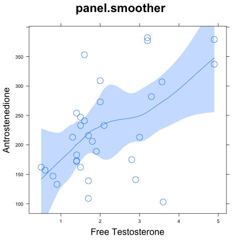
We started on this
analysis because the loess curve seemed to indicate a positive
relationship. We can now be confident in that inference, but there is
still room for skepticism about the detailed pattern. How reliable is
the loess curve itself? To find out, we can put error bounds around
the curve. First the default method of panel.smoother:
xyplot(a~freet, data=h) +
layer(panel.smoother(x,y,degree=1,span=2/3))
The result is shown to the right. I can't figure out how this error
bound is calculated or what it really means, so I suspect it's based
on normal theory. For this reason, I don't trust it when there are
outliers such as those in the present data.
Let's do it a different way, using the bootstrap. I've written a
function for this purpose, which you can get through the "R Source
Code" link on the main course web page. Alternatively, just use the
following "source" statement:
source("http://www.anthro.utah.edu/~rogers/datanal/R/scatboot.r")
This next line does the bootstrap replicates and calculates the upper
and lower confidence bound at each point on the horizontal axis.
sb <- with(af, scatboot(freet, a, confidence=0.90, degree=1,span=2/3))
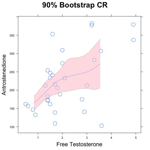 Finally, we call
 scatboot.plot to plot the result:
scatboot.plot(sb, xlab="freet", ylab="a")
The result is shown to the right. The confidence region there is
truncated at the right because there are too few points there to
calculate a 90% confidence region. It is possible, however, to
construct a 75% region: try it.
Exercise
This exercise will involve the msleep data set, which contains
several sleep-related variables scored in a variety of species of
mammal. It's provided with the ggplot2 package, but don't use the
command library(ggplot2): there is a layer function in ggplot2
which may mask the one in latticeExtra. Use this command instead:
data(msleep, package="ggplot2")
That will put a copy of msleep into your workspace without loading
ggplot2 into your search path. You'll also need the quanttst and
scatboot functions, which you can load directly from the web server
like this:
source("http://www.anthro.utah.edu/~rogers/datanal/R/quanttst.r")
source("http://www.anthro.utah.edu/~rogers/datanal/R/scatboot.r")
The quanttst program does the same calculation that you did in a
previous lab project: a permutation test of the hypothesis that two
samples are drawn from the same population, using as a test statistic
the sum of the absolute difference between quantiles. You are welcome
to use your own code if you prefer. If you use mine, the call should
look something like this:
tail.prob <- quanttst(x, y, pr=c(0.1, 0.25, 0.5, 0.75, 0.9),
                      nreps=1000)
The pr argument specifies the quantiles to be used, and nreps is
the number of random permutations to do.
In the msleep data, the sleep_total variable measures the total
time the animal spends sleeping. The vore variable divides the
species into groups, with values such as "omni" (for omnivore) and
"herbi" (for herbivore). Use these data to ask whether omnivores and
herbivores differ in the time they spend sleeping. Attack this
question using (a) a quantile-quantile plot, (b) a t-test, and (c) a
permutation test using the quanttst function (or your own code) with
f-values 0.1, 0.25, 0.5, 0.75, and 0.9. Based on these results,
discuss how total_sleep differs between omnivores and herbivores.
The rest of this exercise involves the relationship between two
variables (sleep_rem and sleep_total) among omnivores. Rem sleep
is the stage of sleep in which dreams happen, so we are asking whether
animals that sleep a lot also dream a lot. To get a sense of these
data, make a scatter plot, with sleep_rem on the X axis, and draw a
loess curve through it. Comment on what you think you see. Is there
a relationship here?
Use the cor.test program to test for a significant association
between these variables. Try all three methods: pearson, spearman,
and kendall. Bear in mind that the pearson method assumes that the
observations are drawn from a bivariate normal distribution. Save
comments until later.
Do a permutation test of the hypothesis that Pearson's r equals 0.
(You don't need to worry now about the normality assumptions, because
the permutation test makes no such assumption.) Save comments until
later.
Use the boot method of the boot package to construct a BCa
confidence interval for Pearson's r. Save comments until later.
Use scatboot to construct a bootstrapped confidence region for
the loess curve with degree=1 and span=2/3. Make two graphs, one for
confidence=0.5 and the other for confidence=0.95. Save comments until
later.
Write a paragraph summarizing these results. Comment both on the
association between the two variables and on the consistency (or
inconsistency) of the results.