Lexicon of Terms

By Robert G. Kent & Tammy  Stump

Largely based on Appendix A: Glossary of Terms from

Butner, J.E., Gagnon, K.T., Geuss, M.N. Lessard, D.A., & Story, T.N. (10/13).  Utilizing topology to generate and test theories of change.  Revise and Resubmit at Psychological Methods.  

• Anti-phase: Movement or change  of components of a system in opposite phase. An example would be the two sides of a rope in a  pulley. As one side moves up, the other side moves down. See an example.
• Attractiveness: The degree to which a system or variable changes towards an  attractor in time; see Lyapunov exponent.
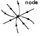
• Attractor: A state that a system or variable changes towards in time. These may be fixed-point (attractive toward one value), periodic (attractive toward a repeating set of values), or strange (attractive toward complex patterns through time). Formerly referred to as a node or a sink.

• Change score: Numerical value of the difference between states; difference  score. This is the simplest representation of a discrete derivative. For example, a change score in systolic blood pressure could show the difference between a measurement taken during a stressor task and a resting baseline reading (e.g., 135-104=31).
• Characteristic root: Strength of a topological feature; see Lyapunov exponent.
• Control parameter: Variables that have the capacity to alter the topology of a  state space. An example would be the temperature of a burner on a stove. At a low temperature, you might let your hand go near the burner, but at a high temperature, you would be less likely to hold your hand near the burner. Control parameters are often thought of as the independent variables of a dynamical system.
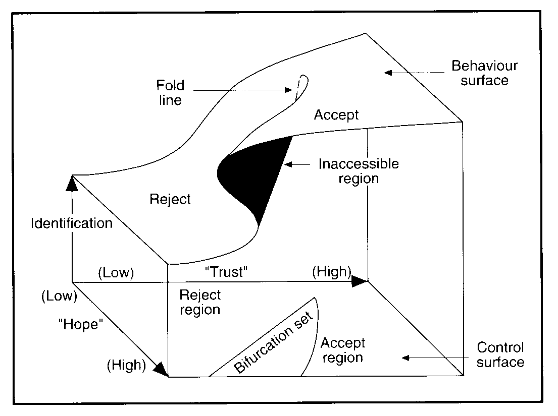
• Cusp catastrophe: A mathematical model in which a system can sometimes show smooth changing behavior and other times show category-like stable states. These states tend to be resistant to change while the smooth behavior tends to function more fluidly. An example would be how attitudes change frequently when they are of low relevance to an individual but when highly relevant they can lock in at high or low values and are resistant to change. In the figure below, the cusp is prominently visible in the center of the topmost plane. It demonstrates that, at certain values of trust and hope, a sudden shift occurs between rejection and acceptance.

Patricia Karathanos, M. Diane Pettypool, Marvin D. Troutt, (1994) "Sudden Lost Meaning: A

Catastrophe?", Management Decision, Vol. 32 Iss: 1, pp.15 - 19

• Damping: Decrease in oscillations of a system. Friction is damping for a moving object.
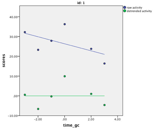
• Detrending: Data processing technique that separates long-term changes from short-term changes. This usually involves calculating a moving average or general pattern of change like a growth model and only retaining the residuals from this model as the data of analysis.  The figure below shows measurements of activity across time in both raw and detrended forms. In the raw data, a negative growth trend is apparent. Detrending removes the pattern across time while retaining the relative association of the scores to the mean and to each other.

• Dynamical systems: The study of dynamics. Multi-component systems that interact to form emergent complex patterns of change over time. An example is weather. Many factors such as temperature, humidity, and air pressure may interact to form a storm.  
• Dynamics: Change over time.
• Equilibrium: State of a system where all influencing forces are balanced and no change (or dynamic order) is occurring.  Most dynamical systems are described as being far-from-equilibrium.  In these systems, energy is flowing into the system and the order of the system constrains the flow of energy, leading to system stability.
• Event sampling: A sampling method where measurements are taken when a  certain event occurs. An example would be filling out a brief series of questions  whenever a person has a social interaction longer than 1 minute.
• Fixed point attractors: The state that a system changes to be closer to a set  value. If a system state is at a fixed point attractor, it will be stable. An example is a pen lying on the ground. A small bump in any direction will most likely result in a pen lying on the ground. The figure below shows movement toward a fixed point attractor in a phase space and a time series.

• Fixed point repellers: The state that a system changes to be farther away from a set value. A system is unstable at the location of a fixed point repeller. It is extremely rare to directly observe a fixed point repeller. An example would be a pen balanced on its tip – a small change in any direction would make it fall. Graphically, fixed point repellers are identical to fixed point attractors with the directionality reversed (i.e., values move away from the point over time).

• Flow: Change of a system. An example would be the movement of a drop of water flowing down a hill.
• Homeostatic: The tendency to maintain stability or return to a set point after perturbation. An example would be the activity of a thermostat. A thermostat activates heating and cooling systems to maintain a specified temperature.
• Homogeneity of model: A model is unchanging in its description across people; see stationarity.
• In-phase: Completely in sync. An example would be the wheels of car when moving straight. Both wheels turn together at the same time and same rate. See an example.
• Interindividual variability: Variability between two or more individuals. An example would be personality. People with different personalities would behave differently. There would be a typical range of personality among a population.
• Intraindividual variability: Variability within one individual. An example would be mood. An individual’s behavior would vary depending on their mood. An individual would have a typical range of mood.
• Latent variables: Variables that were not measured usually captured through Structural Equation Modeling; see also Unobserved Variables.
• Lag: The time period between one event and another. In dynamical systems, the lag between two time points is often used to model the change of a system over time depending on the earlier state. An autoregressive relationship is one form of lag relationship. Also known as a time delay approach.

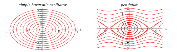
• Limit cycles: A topological feature of a state space in which a system changes in a constant repetition. An example would be the seasons.
• Lyapunov exponent: The numerical value of the strength of a topological feature (such as an attractor or repeller). The rate that a system will change towards or away from a particular state. In geographical terms, this would be the steepness of a slope that a marble is rolling down. Lyapunov exponents can be calculated locally (e.g. at a set point) or globally for the entire system. Global Lyapunov exponents are useful for identifying certain complex behaviors (e.g. deterministic chaos).
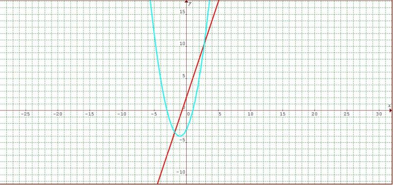
• Nonlinear: In mathematics, an equation in which the terms are not of the first degree/order. The notion of nonlinear has generated some confusion in that a first order model predicting change can generate a nonlinear pattern of change through time. We specifically use nonlinear to depict the predictor side of the equation. By adding polynomial forms and interactions the change equations become able to depict more than one stable pattern with the same equation. The figure below shows a linear (red) and nonlinear (blue) equation. In this case, the nonlinear equation is quadratic.

• Null cline: Area where only one outcome is changing at a time. In terms of equations, the line in which change is fixed to zero while ignoring the other equations in the model. There are as many null clines and dimensions to the topology.
• Order parameter: A variable or set of variables that are sensitive to different phases of a system through their temporal and spatial variance. For example, blood pressure is an order parameter in an ambivalent relationship system--it fluctuates in response to changes in the control parameters of the system.
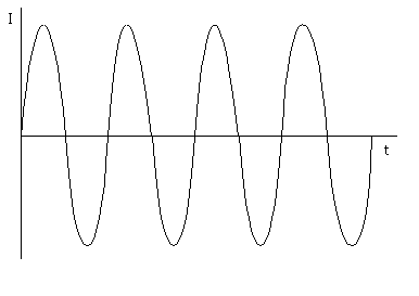
• Oscillation: Repetition of a system’s state over time, as shown below. A pendulum swinging back and forth is a classic example of oscillation.

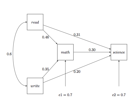
• Path diagrams: A diagram specifying the influence of different parameters on  other parameters of a system, often used in Structural Equation Modeling.  The example shown in the figure below illustrates the predictive power of variables on science achievement.

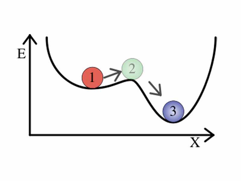
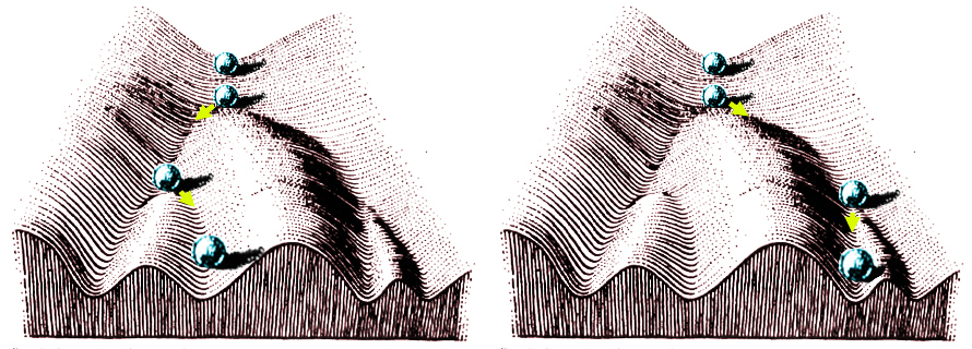
• Perturbation: Small changes in a system due to parts of the system that are necessary, but not modeled. They distinguish the stability of a set point in that an attractor is resistant to perturbations while a repeller is not. This can be seen in the figure below. A slight perturbation could disturb ball 1, but it would settle back into the bottom of the attractor in which it currently rests. Ball 2, by contrast, would be displaced far from its current position by even a tiny perturbation, as the part of the system where it is shown is a repeller. Ball 3 would require a large perturbation to move it out of the basin of the strong attractor where it is currently placed.

• Phase portrait: (not to be confused with phase space): A topographical representation of a state space or phase space where the altitude dimension represents the length of vectors. It is calculated by taking the integral of the equations that generate the state space. Two examples are shown below.

• Phase space: See state space.
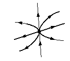
• Repeller: An unstable state that a system or variable moves away from in time.

• Repulsiveness: The degree to which a system moves away from a state; see  Lyapunov exponent.
• Saddle: (or separatrix, pl. separatrices) Topological feature of a state space in which a system is attractive in  one direction and repulsive in the other. An example would be a triangle shaped roof. Rain would drip in one direction on one side of the ridge and drip in the other direction on the other side of the ridge. A saddle is shown near the top of the figure below.  

• Self-organization: A common feature of systems, where elements within the system influence each other, creating order in the system.
• Separatrix, Separatrices: See saddle.
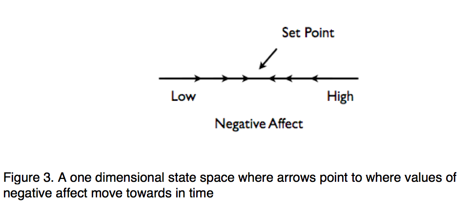
• Set point: A topological feature upon which changes in a system can be  depicted relative to that point. The set point can be defined in Cartesian coordinates of the variables that are changing in time. An example would be the temperature setting of a thermostat. When the temperature rises or falls, the thermostat activates systems to return the temperature to the set point (in this case the set point is an attractor).

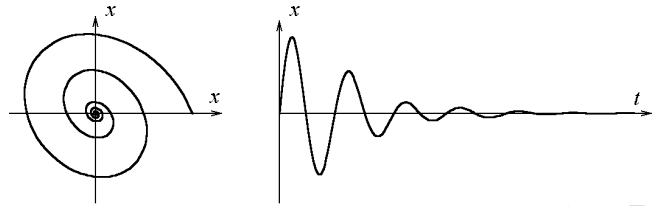
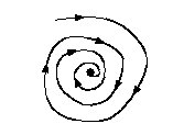
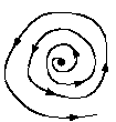
• Spiral attractor: A topological feature that combines a fixed point attractor with a limit cycle so that the state of the system spirals towards a set point.

• Spiral repeller: A topological feature that combines a fixed point attractor with a limit cycle so that the state of the system spirals away from a set point.

• Stable state: A state from which a system is not likely to change. An example would be a marble in the bottom of a Champagne flute. The marble is not likely to move away from its current location. These could be attractors (or example), but they can also be patterns such as the limit cycle.  In the figure below, 1 and 3 are stable (3 is more strongly stable, i.e., is a stronger attractor), and 2 is unstable. A system such as this (exhibiting multiple stable states) is multistable.

• State space: A visual graph of arrows that show where values change over time given where they start. Unlike a time series, time is integrated into the Figure rather than being explicit. State spaces can be hypothetical (what our theory translates into in terms of our expectations of change), observed (plotting an arrow of each observed change), or implied by equations.

• Stationarity: A statistical model that is unchanging in its description of a phenomenon through time; see homogeneity.
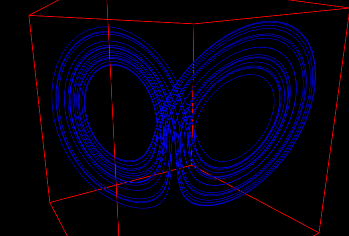
• Strange Attractor: an attractor demonstrating fractal structure. Strange attractors are often (but not always) chaotic. The strange attractor shown here in blue  is the Lorenz or “Butterfly” attractor.

• Strength (of topological feature): The degree to which a system changes towards or away from an area of the state space; see also Lyapunov exponent.
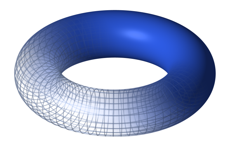
• Taurus or torus: Three-dimensional ring/donut shape. Two second-order equations may specify this shape as a topological feature in a state space.

• Topological feature: A specific pattern of change within the state space of a system.
• Topological map: Graphical representation of a set of equations.

• Topology: The mathematics for linking maps in the form of state spaces and phase portraits to equations of change. All the equations generated are forms calculus that can be expressed with different orders of derivatives as the equation forms.
• Trajectory: Direction towards which a state is changing.
• Unobserved variables: Variables that were not measured; see also Latent  Variables.
• Vector field: See state space.
• Velocity flow field: See state space.

Typical Plots in Dynamical Systems

Below are various types of plots which commonly occur in dynamical systems papers. Unless linked to another original source, the figures below are also reproduced from:

Butner, J.E., Gagnon, K.T., Geuss, M.N. Lessard, D.A., & Story, T.N. (10/13).  Utilizing

topology to generate and test theories of change.  Revise and Resubmit at

Psychological Methods.

There are two main classes of diagrams that are used in dynamical systems: state space plots and phase portraits.

State space plots 

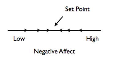
In this figure, the central set point is an attractor, indicated by incoming arrows on either side:   >  < . Low and high negative affect are repellers, as shown by the outgoing arrows moving away from the ends of the line. If a repeller were present in the middle of the data range, it would be shown as a coupled pair of outgoing arrows <  >  .

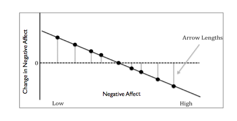
This figure represents the same information that was displayed in the previous plot, but emphasizes the strength and direction of change in negative affect that occurs at specific values of negative affect.  The slope of the line is negative, indicating the presence of an attractor.  At the leftmost point on the line, we see relatively large, positive changes in negative affect.  At the rightmost point on the line, we see relatively large, negative changes in negative affect.  In either case, values are moving closer  the set point (where change is 0).

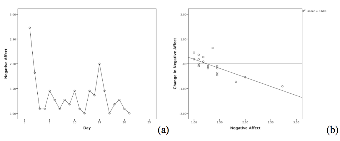
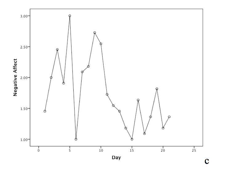
In these plots, we see how a state space plot is created from a person’s data.  Plot a is a time series representation of a single person’s negative affect over 21 days.  To create plot b, for each day, next-day negative affect (using a lag function) is subtracted from same-day negative affect, yielding scores that represent change in negative affect.  Plot b displays these changes in negative affect as a function of negative affect.  Note that time is not included in this plot; the emphasis is on what changes occur at particular levels of the variable.

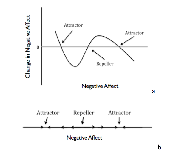
These state spaces show multiple features, 2 attractors and 1 repeller.  Attractors are indicated by line sections with a negative slope in plot a, and by arrows that point toward each other in plot b.  Repellers are indicated by line sections with a positive slope in plot a, and by arrows that point away from each other in plot b.

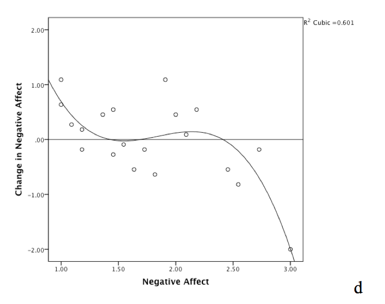
Plots c and d show an example of state space from one person’s data where 3 features (2 attractors and 1 repeller) are present.  As in the one-dimensional example, to create the state space plot, for each day, next-day negative affect (using a lead function) is subtracted from same-day negative affect, yielding scores that represent change in negative affect.  Plot d displays these changes in negative affect as a function of negative affect. A cubic function is used for the fit line, indicating the presence of three features - in order, one attractor, one repeller, and one attractor.

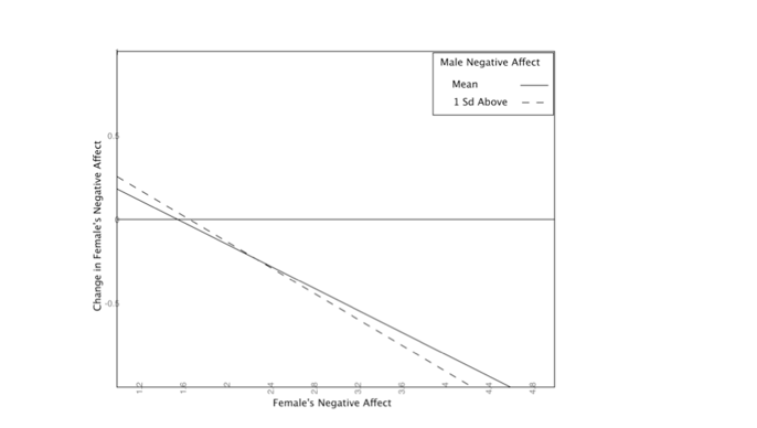
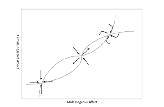
State space plots can also be used to illustrate the effects of control parameters. In this plot, we see that partner’s negative affect changes both the strength and value of the attractor for female negative affect.  When males are higher in  negative affect is  the slope of the line is steeper, meaning the attractor is stronger.  The set point is also slightly higher.

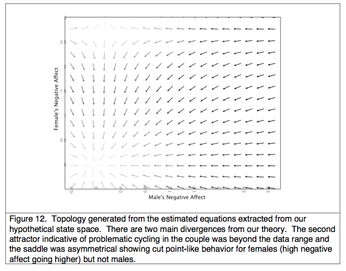
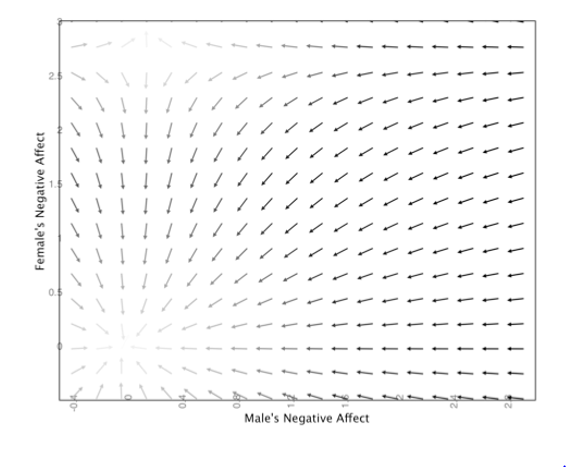
Two-dimensional state space

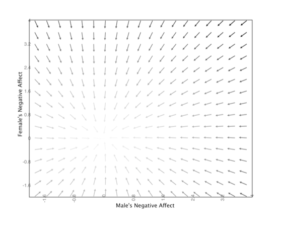
State spaces can also represent changes in more than one variable.  The arrows depict the combination of female and male negative affect that a couple changes to given their current values for negative affect.  Darker arrows indicate larger changes in values.  All arrows moved toward a single point, indicating a fixed point attractor.  Changes are larger when a partner’s affect is farther from the fixed point attractor.

Phase portraits

This figure is a phase portrait of positive and negative affect.  Three features are shown: a fixed point attractor, a saddle, and a spiral attractor.  In light gray, the null clines are depicted; these are the areas where a single dimension does not change.

This is is an epigenetic landscape by Waddington (1957).  In this version of a phase portrait, topological features are indicated by the texture of the surface.   Raised edges represent repellers, while valleys represents attractors.  The positions of the ball represents the current state of the system.  Just as the texture of this surface restricts the flow of the ball, in a dynamical system, attractors and repellers restrict the dynamics of the system. This portrait specifically represents the phenomenon of tissue differentiation.  Once cells begin to organize into one tissue type (in the figure: once the ball reaches one valley), they continue to develop in that manner due to the structure and energy flow within the system.  

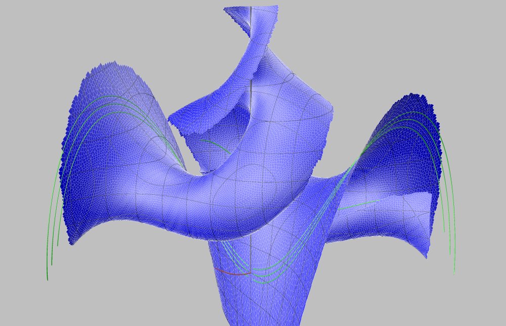
This figure shows a manifold, a space with properties such that the region surrounding any point resembles Euclidian space (i.e., is definable by a coordinate system; see Shelhamer’s 2011 chapter).