Dynamical Systems Theory

Introduction

By Pooja Patnaik & Jeremy Jostad

We live in a world of systems. The natural environment is comprised of multiple types of systems, such as ecosystems. The human body is a system comprised of many interdependent parts (organs, tissues, cells, etc.) that work together which allow us to eat, sleep, and walk on a daily basis. Whether you think of systems in the biological, social, physical, or psychological realm, the fundamental principles are the same. Systems are complex entities that are comprised of multiple working parts that interact with one another to produce behavior (phenomena) that cannot be explained solely by the individual parts alone. We can use these principles beyond the physical or biological realm and apply them to what we, as social psychologists are interested in, human behavior. But what are dynamical systems, you may ask?

First, consider the word dynamic, which simply means change over time. It seems reasonable to assume that systems are not static because even small changes in one component of a system can create large changes in the behavior of the system. However, we are scientists, and we are interested in the ability to measure and predict the behavior of systems. Welcome mathematics! Add an “al” to “dynamic” and you have “dynamical,” which refers to the use of mathematics to measure and model the changes within a system over time. Therefore, dynamical systems theory uses mathematical equations to specify and predict the time-based properties of system phenomena. Fundamentally, it is the patterns of behavior, or the “spatio-temporal dance,” in which we are most interested in understanding. You may be asking yourself, “great, but how is this any different than traditional methodologies?”

Dynamical systems theory is an interdisciplinary theory that combines many different theories, including chaos theory and catastrophe theory. Chaos is a seemingly random and completely unpredictable behavior. Statistically, chaos and randomness are not different. Examples of chaotic systems include physical (weather), social, and economic systems (stock market). To be discussed later, the logistic map equation is a simple mathematical formula that ultimately leads to chaotic behavior.

Chaos is commonly referred to as “a state of disorder”. As a result, it makes sense that chaos is where the ability to predict is limited. Entropy is the ability to predict what is next, based off of everything one knows from before; therefore chaos has low entropy since its ability to predict is limited. In the real world, we usually do not know the state of the world precisely, but only approximately. For example, we can determine a lot about today’s weather by measuring temperature and pressure at a number of locations in the world. But this does not give us complete information- we do not know the velocity or position of every single molecule in the atmosphere. Chaos theory studies the behavior of dynamical systems that are highly sensitive to initial conditions- an effect that is popularly referred to as the butterfly effect. The question is if the flap of a butterfly’s wings in Brazil sets off a tornado in Texas. The flapping wing represents a small change in the initial condition of the system, which causes a chain of events leading to large-scale phenomena. Had the butterfly not flapped its wings, the trajectory of the system might have been vastly different.

Now that you have an understanding of chaos, see if you understand Sheldon’s explanation, below:

http://www.youtube.com/watch?v=eqZyn3I46aM

Catastrophe theory is the study of behavior that has sudden shifts or changes in behavior. In doing so, catastrophe theory has been able to explain, for example, how sudden abrupt changes in behavior can result from minute changes in the control factors and why such changes occur at different control factor configurations depending on the past states of the system. Consider, for example, opening a door that is jammed. As increasing pressure is applied, nothing happens, and the door remains stuck. However, at some point, a miniscule increase in pressure will cause the door to become unstuck. The transition from stuck to unstuck or jammed to un-jammed, is a catastrophe.

Remember that we are interested in the overall macroscopic or emergent behavior of the system. Using ecosystems as an example, we cannot understand how all of the parts of an ecosystem work together to produce a healthy habitat if we are solely focused on the cellular structure of a plant. As system dynamists, we assume there are multiple components within a system that both constrain and produce macroscopic emergent behavior. We are not concerned with trying to measure every component of the system. Rather, we believe a system is best understood by taking a step back and observing the system as a whole. The traditional research paradigm takes a reductionist approach, by seeking to break the system into individual parts to see how each part influences one another. As the reductionist scientist continues to break down the system, they become increasingly detached from the behavior under study. A second difference from traditional methodologies is the non-linear nature of systems. Systems do not behave in a linear fashion. Traditional statistical and analytic strategies, however, model behavior as though it were linear. As we will see throughout this website, system behavior can be relatively stable with large changes within its components, and on the other hand we can see extremely dynamic behavior by small changes within the components of a system. Using equations with non-linear terms will help in measuring and modeling system behavior.

Before moving forward any further, let’s discuss some of the fundamental assumptions of dynamical systems theory. These will be terms and ideas that create the building block of inheriting a systems framework.

Emergence and Self-Organization

Emergence is a fundamental assumption of dynamical systems theory which suggests that the interaction of the components of a system produce a pattern of behavior that is new or different than that which existed prior. Emergence happens every day in our lives. We can see, feel, and touch emergent phenomena. Weather is a great example of emergent phenomena. A hurricane does not simply occur on its own; rather, certain interactions of weather components (temperature, wind, moisture, etc.) interact to produce this phenomenon. The logical question to ask is “how does emergence occur?” As stated above, it is the interaction of the components within a system, however, the notion which specifies how these components interact is known as self-organization.

Self-organization is the process by which emergence occurs. There is not an acting agent within the system that specifies how the components should interact with one another; rather, the interactions are governed by feedback loops. Several key concepts and conditions are important for self-organization in systems:

1) Interactions within systems must be non-linear. Patterns emerge because of the different types and levels of interactions that can occur between the components of the system.

2) A system must be far from equilibrium. This means that a system must be an open system and not a closed system. Although closed systems really only occur in a vacuum, the idea is important. Systems must have a constant flow of energy in and out of the system. If this does not occur, then a system would find its equilibrium and essentially die. In social psychology, we often refer to this “energy” as information.

3) Systems exhibit hysteresis, which literally means “history matters.” The future state of a system will depend on the past and present states.

4) Circular causality is present in systems. The pattern (emergence) is restricted by the behavior of the components of the system, but the components of the system are also restricted by the global patterns.

5) Fluctuations or perturbations are constantly trying to move the system, which will provide an understanding of the stability of various phases. These perturbations should not be misinterpreted as error.

6) The slaving principle acts as a selection mechanism for the interaction of the parts of the system (Kelso, 1995). That is, once the order parameter (see below) is fully developed and rather stable, it “enslaves” the parts of the system into specified interactions.

To understand how emergence and self-organization operate, consider the Raleigh-Benard instability, a classic example of emergence through self-organization.

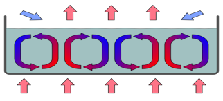
The Raleigh-Benard Instability

The Raleigh-Benard instability demonstrates the emergent behavior or spatio-temporal dance of a liquid when heated from the bottom. Consider a pan with oil inside that is not being heated. If the temperatures within and surrounding the liquid are the same, the molecules are moving about randomly. However, when a source of heat is added to the bottom of the pan, the movement of these molecules begins to change. The molecules that are near the bottom of the pan are warmer and will rise to the top of the surface of the liquid. The cooler molecules are denser and will sink to the bottom of the liquid. At a particular temperature gradient (difference in temperature between the bottom and top of the pan) a pattern emerges within the liquid that is developed by the movement of the molecules (the components of the system). Convection cells within the liquid emerge that create a rolling motion opposite of one another (see Figure 1 below). Through this motion, hexagonal cells emerge in the liquid. Thus, the spatio-temporal pattern of the liquid changes as the molecules transition from a state of disorder into a coordinated whole. At a particular temperature gradient this spatio-temporal dance will remain stable and continue. However, if the temperature gradient continues to increase, the liquid becomes turbulent and transitions into a state of disorder. The Raleigh-Benard instability shows that complex patterns can emerge through the self-organization of the molecules in the liquid. To understand how this system works, do we need to know the pattern of every molecule in the system? Hopefully you said no, because it is the pattern of the liquid in which we are interested.

Figure 1

Click on the link below to watch the Raleigh-Benard Instability in motion:

http://www.youtube.com/watch?v=kJnE12dJ9ic

Sensitivity to Initial Conditions

An important concept to dynamical systems is the notion that non-linear dynamics are sensitive to initial conditions. That is, small initial differences in initial conditions or measurements can lead to vast differences in long-term predictions. This is one of the defining ideas of chaos (Mitchell, 2009) and may best be shown through the logistic map equation. The equation is as follows:

x_t+1 = Rx_t (1-x_t)

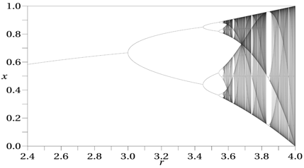
where x_t is the current value of x and x_t+1 is the value at its next step; R is a constant. What this fairly simple equation suggests is that small changes or differences in the value of the constant (R), can have dramatic changes in the long-term behavior. Figure 2 shows a bifurcation diagram for the logistic map. What can be shown here is that fixed points (the straight line in the figure) are reached when R is below about 3.1. At a value of 3.1, the map creates what is called a bifurcation. The predicted value now oscillates between two values. When R reaches a value between 3.4 and 3.5, the period bifurcates again and now the future value oscillates between four different values. The higher we raise the value of R, the periods continue to double until they have reached a chaotic state (which begins when R is approximately 3.569946). These bifurcations represent a phase transition in the state of the system.

Figure 2

A very fun tool can be used to model the logistic map at the following link:

http://old.psych.utah.edu/stat/dynamic_systems/Content/chaos/index.html

Phase Transitions

A phase transition is the transformation of a thermodynamic system from one phase or state of matter to another one. A phase space of a dynamical system is the collection of all possible states of the system in question. A phase transition occurs as a result of some external condition, such as temperature, pressure, etc. For example, a liquid may become gas upon heating to the boiling point, resulting in a change in volume. The measurement of the external conditions at which the transformation occurs is termed the phase transition. The term is most commonly used to describe transition between solid, liquid, and gaseous states of matter.

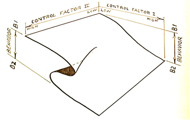
One way that phase transitions can be applied is by studying cusp catastrophe models. The cusp catastrophe model is one of many catastrophe models, which has been applied several times in psychology from areas ranging in binge drinking with attitudes towards alcohol, to speed-accuracy trade-offs, and a general model of attitudes. The model describes how changes in a dependent variable, like behavior, are related to the levels of two independent variables. It is a mathematical model in which a system can sometimes show a smooth changing behavior and other times show stable states. These states tend to be resistant to change while the smooth behavior tends to function more fluidly. There exists two stable states and is generally a function of control parameters. The only stable locations for behavior are assumed to be on the surface. Hysteresis plays a role in that it refers to the predicted tendency for behavior to resist change in spite of the two independent variables’ effect on it. Going back to phase transitions, this means that when experimental settings continuously change and force people to switch from one independent variable to another, the switch will be abrupt.

Figure 3

Characteristics of Dynamical Systems

Stability

Dynamic systems try to achieve and maintain a stable state. When a system is pushed far from equilibrium in seeking stability, it adopts certain patterns which try to achieve local stability. The local stability is reached with the use of order parameters and control parameters. Stability is a resistance to perturbations, which are small changes to or disturbances in the system. The stability of a system can be measured in several ways. First, stability is indexed by the statistical likelihood that the system will be in a particular state rather than other potential states. Second, stability can be measured depending in how it responds to perturbation. If a small perturbation applied to the system drives it away from its stable state, after some time the system will settle back to its original position. Third, stability is related to the system’s response to natural fluctuations within the system. In systems theory, a system in a steady state has numerous properties that are unchanging in time. You might already be familiar with homeostasis, which is the property of a system, either open or closed, that regulates its internal environment and tends to maintain a stable, constant condition.

Order Parameters

Order parameters define the overall behavior of a system by enabling a coordinated pattern of movement to be reproduced and distinguished from other patterns. Order parameters are the phenomena in which we are seeking to understand. Phase transitions occur when order parameters change as a function of another parameter of the system, such as temperature. An order parameter is a measure of the degree of order across the boundaries in a phase transition system. For liquid/gas transitions, the order parameter is the difference of the densities. When a control parameter is systematically varied (i.e. speed is increased from fast to slow), an order parameter may remain stable or changes it stable state characteristic at a certain level of change of the control parameter.

Control Parameters

Control parameters are responsible for changing the stability of states. A control parameter does not control the change in behavior but rather acts as a catalyst for reorganizing behavior. The control parameter does not really “control” the system in traditional terms. Rather, it is a parameter to which the collective behavior of the system is sensitive to and thus, moves the system through collective states. Control parameters lead to phase shifts by threatening the stability of the current attractor. Control parameters are similar to moderators within psychology. Subsequently, systems are concerned about how other variables moderate a variable’s relationship with itself. In the Raleigh-Benard instability discussed earlier, heat is a control parameter as an outside variable pushing the system into different behaviors.

State Space

A state space is an abstract construct which describes the possible states of the collective variable. For example, the behavior of a simple mechanical system, such as a pendulum, can be described completely in a two-dimensional state space where the coordinates are position and velocity and as the pendulum swings back and forth, its motion can be plotted on a plane. The motion of the pendulum has a path through the state space that tracks its regular changes of position and velocity. State spaces can also be constructed in three dimensions.

Topology is the graphical representation of differential equations in three-dimensional space. Topology is generally displayed as an elevation map of some geographical terrain and can be applied more generally to describe anything, like behavior or psychological constructs that change over time. Control parameters have the ability to alter topological features in one of three ways. First, they can strengthen/weaken an attractor or repeller (scroll down for definitions). Second, control parameters can move a set point to a different location relative to other set points. Third, control parameters can drastically change the topology by completely extinguishing set points or turning it into a different kind of topological feature (e.g. change an attractor to a repeller or vice versa).

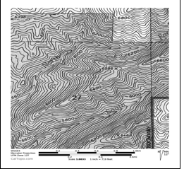
Figure 4 is a picture of a topographic map near the University of Utah. Not only does this map measure distance and direction on the X and Y axis, but it also measures elevation through the lines. Thus, it represents a three dimensional space. Imagine that the X and Y axis represented different constructs. Now imagine that a person was placed somewhere in this geographical terrain. Most likely this person is going to travel in the path of least resistance, down-hill or on relatively flat terrain. The same can be said of the state of the system when using topography. That is, depending on where the current state of the system resides, a topology can tell us the most likely future dynamics of the system. Valleys can represent attractors, whereas hills and peaks can represent repellers, which will be discussed next.

Figure 4

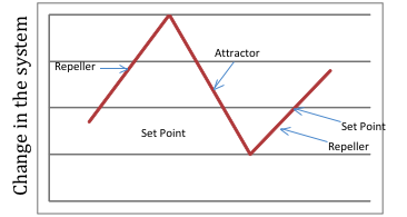
Patterns of Behavior in the System

A critical property of self-organizing, open systems is that, although an enormous range of patterns is theoretically possible, the system actually displays only one or a very limited subset of them. A dynamical system is generally described by one or more differential or difference equations. The equations of a given dynamical system specify its behavior over any given short period of time.

Attractors

In dynamical systems, an attractor is a set of physical properties toward which a system tends to evolve, regardless of the starting conditions of the system. Attractors draw the system toward this state space. If we consider a graph that represents change in the system, an attractor will have a negative slope. A less steep slope indicates that points are moving towards the attractor slower. Think of it as attraction- when you are attracted to someone, you are drawn in by them. A fixed point attractor is in two dimensions which can be thought of as a combination of two people’s behavior drawn together (as if both of the people below are running towards each other). In 3D, you find spiral attractors (more below).

Repellers

If a set of points is periodic or chaotic, but the flow in the neighborhood is away from the set, the set is not an attractor, but instead a repeller. Repellers are more theoretical, rather than observed as they serve as boundaries between attractors. Graphically, a repeller has a positive slope. A steeper slope indicates that the points are moving away faster. Taking the analogy from above, if you are ‘repulsed’ by someone, you try to move away from them. A fixed point repeller is in two dimensions as well where you can think of it as a combination of two people who are repulsed by each other (as if both of the people below are running away from each other). Similar to attractors, in 3D, you find spiral repellers.

Set Points

A set point is where all behavior in a system is depicted in relation to this point. Attractors move towards the set point whereas repellers are driven away from this point. These are generally points of no change. When dealing with oscillations, it is the point the system oscillates around (remember, the point of zero change).

Figure 5

Periodicity

Periodicity of the system measures the manner in which a system returns regularly to the same state (or similar state) because of a pattern that repeats ad infinitum. Periodic behavior can be defined as recurring at regular intervals, such as “every 24 hours”; the amount of time it takes to complete one cycle is a period. Earlier, we talked about chaos’ low entropy due to its limited predictability; therefore periodicity has high entropy since there’s a high ability to predict the future since there is a repeated pattern. A dynamical system exhibiting a stable periodic orbit is often called an oscillator. An oscillation is a repetitive variation between two or more different states, like a swinging pendulum.

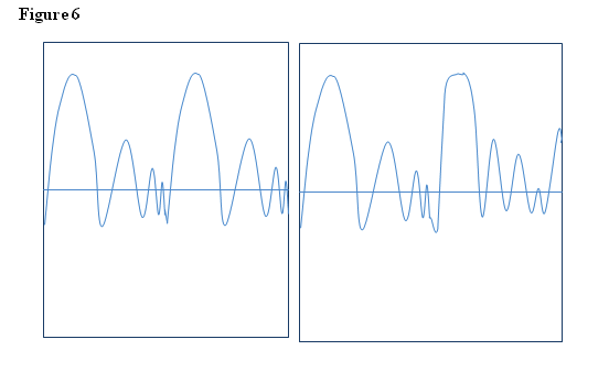
Quasi-periodicity is the property of a system that displays irregular periodicity, so it is a set that nearly repeats. Take a look at the graphs in Figure 6. The graph on the left displays periodicity in that the same pattern will repeat forever if nothing stops the movement, and the graph on the right displays quasi-periodicity because the oscillations may be similar, but they’re not exact. The repetition is not perfect like a periodic system but it has similar repetitions. Quasiperiodic behavior is a pattern of recurrence with a component of unpredictability that does not lend itself to precise measurement.

Figure 6

Limits

Limit cycles have been used to model many real world oscillatory behaviors over time. A pendulum that is not affected by friction will repeat its oscillations forever, which is known as a limit cycle, since the system changes in a constant repetition, but does not necessarily repeat the same value every time. Stable limit cycles imply self-sustained oscillations: the closed trajectory describes perfect periodic behavior of the system. Any small perturbations from this closed trajectory cause the system to return to the limit cycle.

Combining limit cycles with other elements allows for many other possibilities that expand the topology. For example, spiral attractors (spiraling towards the set point in time) occur by combining a fixed point attractor with a limit cycle. Similarly, a spiral repeller is where a fixed point repeller is combined with a limit cycle.

A limit set is the state a dynamical system reaches after an infinite amount of time has passed, and is important because they can be used to understand the long-term behavior of a system. Attractors are limit sets but not all limit sets are attractors. For example, if a pendulum is losing its speed and point X is minimum height of the pendulum and point Y is the maximum height, point X is a limit set because the trajectories move towards it and point Y is not. In addition, since the pendulum is losing speed, point X is an attractor.

Lyapunov exponents

We have talked about the different ways a system can potentially move towards stability but what do we do when we want to know how chaotic the system is? A Lyapunov exponent can tell us how chaotic a system is by merely quantifying the degree of and characterizing the extent of the sensitivity to initial conditions. It is a numerical value that captures the rate of entropy for a given topological representation of the data (the steepness of an attractor or repeller). To identify a Lyapunov exponent, we need to identify the change that occurs just off the set point. There is a whole spectrum of Lyapunov exponents and the number of them is equal to the number of dimensions in the phase space (e.g. if we are studying a system in 4 dimensions, there will be 4 Lyapunov exponents).