Catastrophe Models in Multilevel Modeling
Jonathan Butner
In Dynamical Systems Theory, few models
capture (most of) the notions of dynamics better than the catastrophe
models from Catastrophe Theory. The catastrophe models are a
series of equations that incorporate multistability and control
parameters in one. The most commonly discussed catastrophe model
is the cusp catastrophe. The cusp catastrophe is capable of depicting a
measure that sometimes functions continously and sometimes discrete. And it
illustrates how a variable can moderate a system - turning a single
attractor into a pair. More complex (and simpler) catastrophe
models exist. I will review a little bit of background, focus on
the cusp catastrophe model in particular, and then show how this
translates into a multilevel modeling circumstance. Finally, I
will review some issues that need addressing for this multilevel
modeling approach.
Attraction and Repulsion
Attraction and Repulsion
The notion of attraction and repulsion
in systems theory is pretty straight forward, but with some hidden
assumptions. An attractor merely means you move towards something
and a repeller means you move away. We say that attractors are
stable because if you begin to move away from the point of attraction
(assuming a fixed point attractor, there are other kinds of attractors
too), you move back. We say a repeller is unstable because if you
begin to move away from the point of repulsion, you continue to move
away. Note that both fixed point attractors and fixed point
repellers have a point you can sit at and not move, in theory. In
reality this never happens for the repeller.
So here is where perturbations come in. If we envision an open system of which we are depicting the big systematic components, the remaining components that we are failing to capture come out as constantly knocking around the system through time - perturbations. Systems are constantly being perturbed because we cannot capture everything, just a large chunk of it. We define something as stable because we continue to observe the behavior despite these perturbations. A fixed point attractor is stable because we see hovering around the fixed point despite the constant onslaught. A repeller will pretty much always result in moving away patterns and nothing more, because of that very same onslaught.
We can see the notion of attraction by displaying this time series as a scatterplot, but where the Y-axis is Change in X and the variable (in raw metric) on the X-axis.
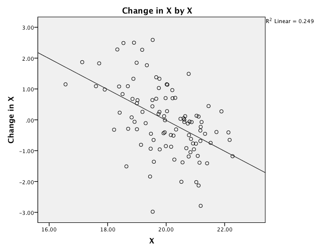
The angled line is the linear least squares slope. This is the equation I actually used to generate this:
Change in X = b0 + b1X + e
When the slope (b1) is negative, we get an attractor. When the slope is positive, we get a repeller. The steepness of the slope indicates the strength of attraction/repulsion. I have a video series that explains this in detail. As noted in the video series, the key is identifying the set point (the point of no change) and describing behavior relative to the set point. In this case, since the line is a straight line, the strength is a linear function of the distance from the set point.
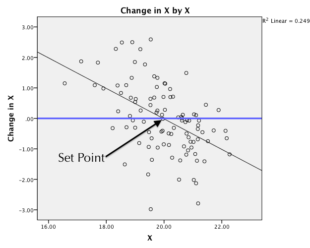
Cusp models (as we will cover below) will make a nonlinear relationship between change and outcome. So, it is easiest to evaluate behavior at the set point(s) - examining the location and the slopes at each of the set points to determine the behavior.
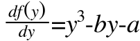
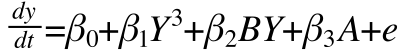
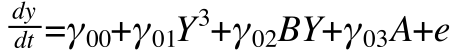
The df(y)/df is some function of the change in Y, usually in terms of a derivative or difference form. I am going to replace this with change in Y (first derivative), though there is no reason we could not use other derivatives of difference forms (in fact, there are some very interesting insights into classic oscillatory terms when couched this way, but that is for another day). Additionally, I am going to flip all the signs because it is a little easier with which to work.
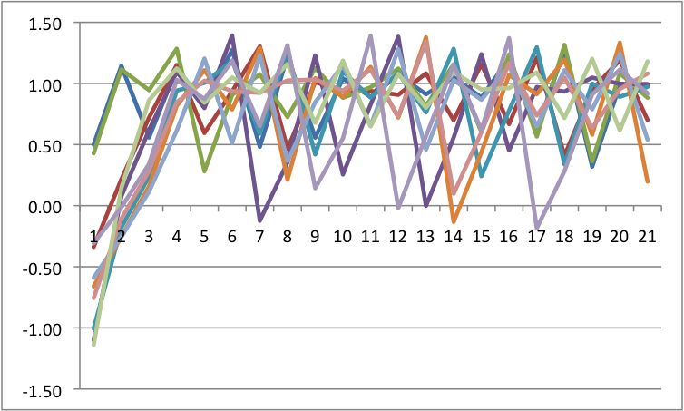
Note that there are two other parameters in the equation, A & B. These are the control parameters and they moderate the strength, location, and multistability vs unistability of the attractors. I simulated some data circumstances to see how this works. I am going to live in a standardized world for a moment (later I will criticize standardization for this kind of procedure, but it will not matter for my simulations). Let's imagine four scenarios: When A and B are low; When A is low and B is high, when A is high and B is low, and finally when both are high. In each case, I am starting with the same initial values and generating a bunch of time series (without perturbations).
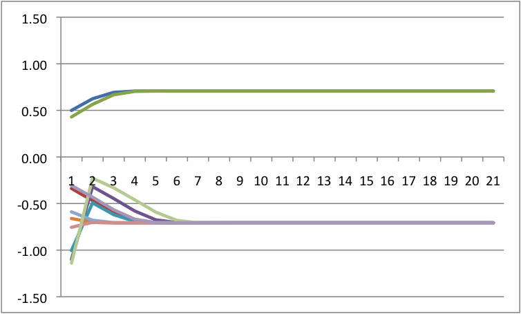
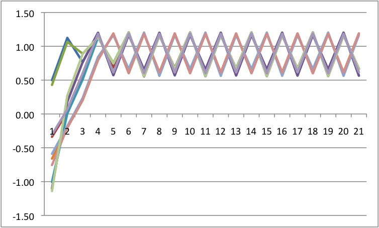
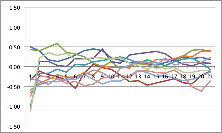
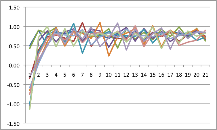
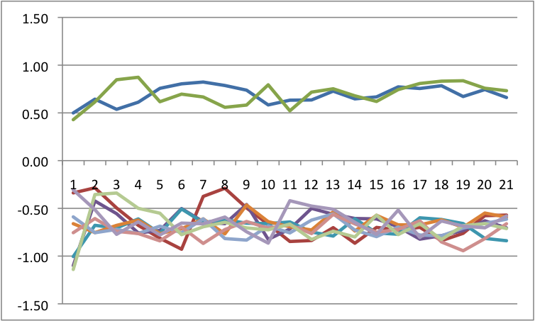
Recall how I said perturbations are key? I am now going to add perturbations to each because it will have differential impact. The way I am doing this is that I am adding a random, normally distributed number to the change in Y at each point in time. I have scaled the size of these numbers down so that they are big, but do not overwhelm the system. Across all of these, I will force the same random numbers so that only the differences are a function of control parameters.
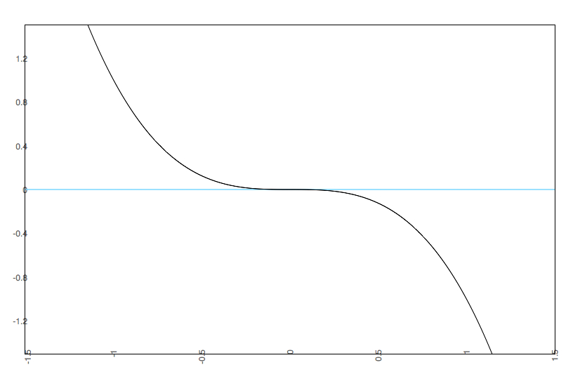
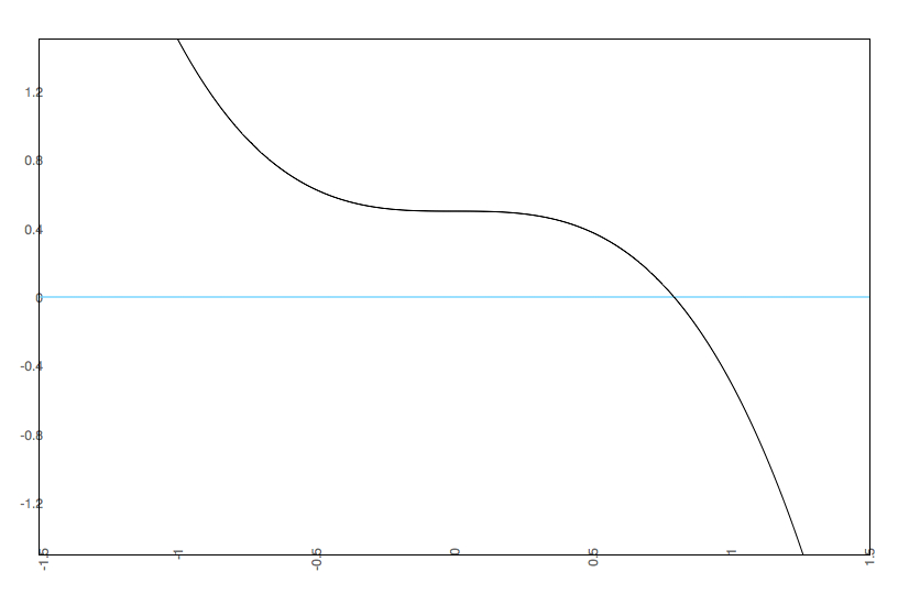
Notice that we see multistability on the bottom left. To get an easier understanding of what is going on, below is the predicted plots placing change on the Y axis, and value on the X axis with A & B at their fixed values.
Notice that we are going from one set point to three set points. In the one set point case (b=.5 & a=.5 or b=0 and a= anything), there is a single attractor. In the three set point case (b=.5, a=0), the slopes go negative, then positive, then negative. That is, there is a pair of attractors with a repeller separating them. A is known as the bifurcation parameter - it determines when there are one or two attractors. B is known as the asymmetry parameter - when there are two attractors it determines the relative strength of each attractor.
The Cusp Surface and Other Graphical Representations
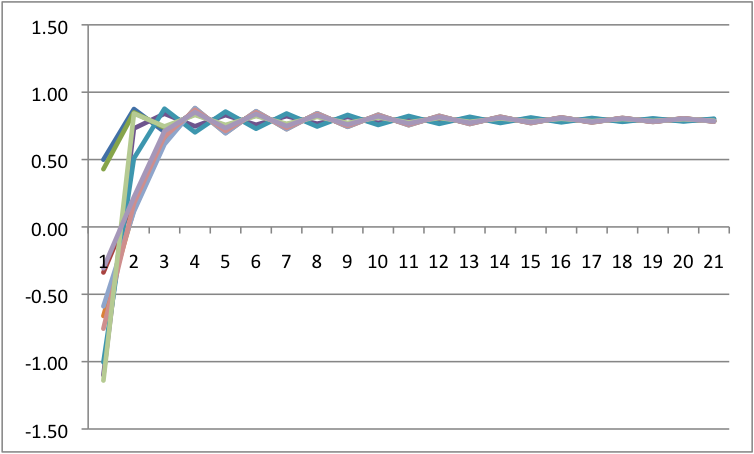
The common representation for the cusp catstrophe model is the surface plot of the values for Y that are stable.
The surface is a great way to illustrate the full series of relationships. In this case, the Y axis is our outcome and the two control parameters are the X (b) and Z (a) axes.
We can also illustrate the cusp catastrophe model through potential wells (also known as potential energy wells). These are the integral of the cusp catastrophe equation times a negative constant such that a lower value on the Y axis represents less potential for change. As with my table of four figures above, we would expect different potential wells at different levels of A & B.
The way to read the potential wells is to imagine a marble dropped into the bowl. The X axis is the value of the outcome and the Y axis is the potential for change. So, it is just like a bowl in that you envision where the marble will roll in time. Perturbations are then little flicks against the marble pushing it left and right. Only in the lower left do we see two bowls.
Perturbations are a Necessary Concept
Attraction and repulsion (or more specifically, stability/instability) cannot be defined without perturbations. There is a key difference between idealized systems and the reality of systems we study, and that distinction boils down to closed vs. open systems. A closed system (in the most general sense) merely means that we have everything measured that is involved in the system. A physicist would say that the total energy is a constant. An open system merely means that we are measuring some portion of the system. A physicist would say that there are injections (known as escapements) and loss (known as damping) of energy from/to the parts of the system not being examined. A closed system says we have created representation of the entire system, while an open system says that we will never fully depict the entire system, just the big systematic components.So here is where perturbations come in. If we envision an open system of which we are depicting the big systematic components, the remaining components that we are failing to capture come out as constantly knocking around the system through time - perturbations. Systems are constantly being perturbed because we cannot capture everything, just a large chunk of it. We define something as stable because we continue to observe the behavior despite these perturbations. A fixed point attractor is stable because we see hovering around the fixed point despite the constant onslaught. A repeller will pretty much always result in moving away patterns and nothing more, because of that very same onslaught.
Now In Regression
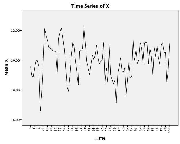
A fixed point attractor can be captured in a simple regression equation!! Imagine that we have a single time series. Through time, an attractor is going to look like a bunch of points all hanging around that one value. Here is a simulated time series. I will show you the equation in a moment.We can see the notion of attraction by displaying this time series as a scatterplot, but where the Y-axis is Change in X and the variable (in raw metric) on the X-axis.
The angled line is the linear least squares slope. This is the equation I actually used to generate this:
Change in X = b0 + b1X + e
When the slope (b1) is negative, we get an attractor. When the slope is positive, we get a repeller. The steepness of the slope indicates the strength of attraction/repulsion. I have a video series that explains this in detail. As noted in the video series, the key is identifying the set point (the point of no change) and describing behavior relative to the set point. In this case, since the line is a straight line, the strength is a linear function of the distance from the set point.
Cusp models (as we will cover below) will make a nonlinear relationship between change and outcome. So, it is easiest to evaluate behavior at the set point(s) - examining the location and the slopes at each of the set points to determine the behavior.
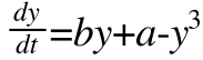
The Cusp Catastrophe
The cusp catastrophe builds on the attractor notion by allowing for more than one attractor at the same time (multistability), but also moderators that modulate when there is a single attractor or two different attractors (control parameters). There is a very elegant color based teacher for the cusp catastrophe that I highly recommend exploring. I am going to work from the regression equation perspective. The equation for the Cusp catastrophe model follows (taken from Guastello, 2010):The df(y)/df is some function of the change in Y, usually in terms of a derivative or difference form. I am going to replace this with change in Y (first derivative), though there is no reason we could not use other derivatives of difference forms (in fact, there are some very interesting insights into classic oscillatory terms when couched this way, but that is for another day). Additionally, I am going to flip all the signs because it is a little easier with which to work.
Note that there are two other parameters in the equation, A & B. These are the control parameters and they moderate the strength, location, and multistability vs unistability of the attractors. I simulated some data circumstances to see how this works. I am going to live in a standardized world for a moment (later I will criticize standardization for this kind of procedure, but it will not matter for my simulations). Let's imagine four scenarios: When A and B are low; When A is low and B is high, when A is high and B is low, and finally when both are high. In each case, I am starting with the same initial values and generating a bunch of time series (without perturbations).
 b=0 a=0
|
 b=0 a=.5 |
 b=.5 a=0 |
 b=.5 a=.5 |
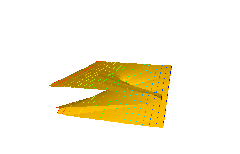
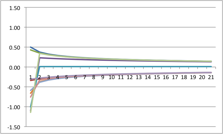
Recall how I said perturbations are key? I am now going to add perturbations to each because it will have differential impact. The way I am doing this is that I am adding a random, normally distributed number to the change in Y at each point in time. I have scaled the size of these numbers down so that they are big, but do not overwhelm the system. Across all of these, I will force the same random numbers so that only the differences are a function of control parameters.
 b=0 a=0 |
 b=0 a=.5 |
 b=.5 a=0 |
 b=.5 a=.5 |
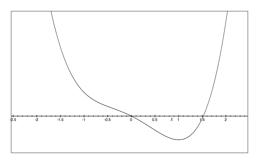
Notice that we see multistability on the bottom left. To get an easier understanding of what is going on, below is the predicted plots placing change on the Y axis, and value on the X axis with A & B at their fixed values.
 b=0 a=0 |
  b=0 a=.5 |
 b=.5 a=0 |
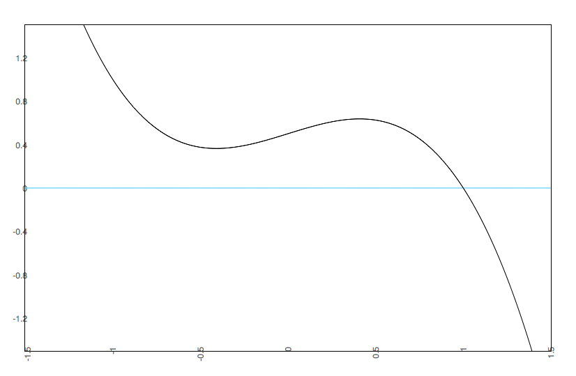 b=.5 a =.5 |
Notice that we are going from one set point to three set points. In the one set point case (b=.5 & a=.5 or b=0 and a= anything), there is a single attractor. In the three set point case (b=.5, a=0), the slopes go negative, then positive, then negative. That is, there is a pair of attractors with a repeller separating them. A is known as the bifurcation parameter - it determines when there are one or two attractors. B is known as the asymmetry parameter - when there are two attractors it determines the relative strength of each attractor.
Having A & B Change Through Time
Up until now, I have kept A and B at one constant value or another. However, the cusp catastrophe model can allow A & B to be changing. In fact, common applications of the catastrophe model always assume these can be altering values over time and people. This will be important when we get to multilevel modeling. In my table of figures above (with the four panels), at any given instance in time the A and B should determine the behavior. It is common to assume that A & B are normally distributed and independent through time, which is probably unrealistic. It also probably does not hurt us to assume this though.The Cusp Surface and Other Graphical Representations
The common representation for the cusp catstrophe model is the surface plot of the values for Y that are stable.The surface is a great way to illustrate the full series of relationships. In this case, the Y axis is our outcome and the two control parameters are the X (b) and Z (a) axes.
We can also illustrate the cusp catastrophe model through potential wells (also known as potential energy wells). These are the integral of the cusp catastrophe equation times a negative constant such that a lower value on the Y axis represents less potential for change. As with my table of four figures above, we would expect different potential wells at different levels of A & B.
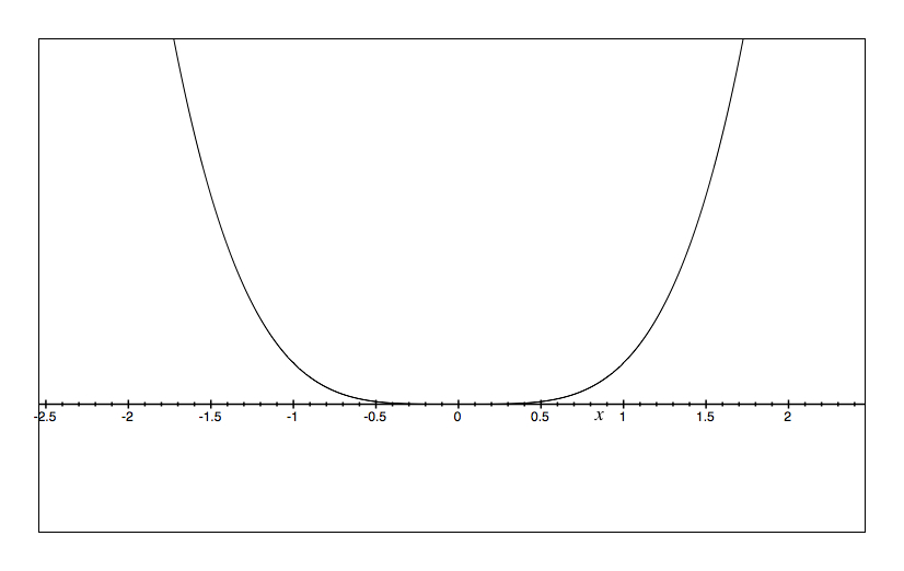 b=0 a=0 |
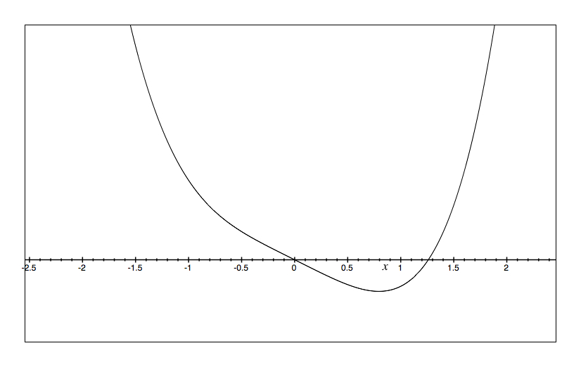 b=0 a=.5 |
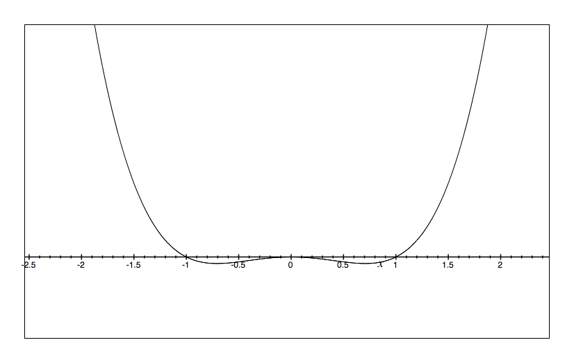 b=.5 a=0 |
 b=.5 a =.5 |
The way to read the potential wells is to imagine a marble dropped into the bowl. The X axis is the value of the outcome and the Y axis is the potential for change. So, it is just like a bowl in that you envision where the marble will roll in time. Perturbations are then little flicks against the marble pushing it left and right. Only in the lower left do we see two bowls.
Multilevel Modeling as Means to the Cusp Catastrophe
In Butner, Dyer, Malloy, and Kranz (In
Press), we illustrate how the cusp catastrophe model can be tested in a
multilevel modeling context. Multilevel modeling (also known as
mixed models, hierarchical linear modeling, and random coefficient
modeling) is a maximum likelihood based procedure designed for nested
data structures. In this case, the nesting is the idea that we
have multiple time series rather than just one. It can be thought
of as an expansion of ANOVA or Regression such that repeated measures
ANOVA is a special case.
Bryk and Raudenbush pointed out that multilevel models are analogous to running a regression within individuals (one for each time series), saving out the regression coefficients and then comparing the coefficients across individuals. They call the equation within cases the Level 1 Equation and the Equations comparing coefficients between cases as the Level 2 Equations. The actual equation tested under Maximum Likelihood is the nested (or mixed) equation where the coefficients in level 1 are replaced with the equations in Level 2. Also, maximum likelihood estimation is an asymptotic estimation procedure. So, estimates are always population based calculation. Thus, error terms are represented by error variances (and a model might have a couple of them known as random effects).
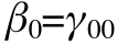
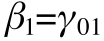
So, let's say that the level 1 equation is the cusp catastrophe regression equation earlier. The only change I will make is to switch to greek symbols because of ML being an asymptotic procedure (greek for population, old statistical norm).
And let's say that the level two equations just had intercepts (no predictors, no residuals). This is like saying that everyone has the identical level 1 equation:
The nested equation (actual equation tested) just combines the level 1 and level 2 equations:
Scaling and Expanding the Equation Form
Now the equation above is imperfect. It is based on the
topological formulation of the cusp catastrophe. It is
mathematically correct, based on a scale free nature. However,
multilevel modeling (and regression too, so what I am about to say
would also apply to the earlier parts) generates partial derivative
relationships. The moment we add interactions and polynomials,
many of the terms lose their scale free nature. To see the issue,
let's go to a much simpler regression circumstance:
Y=b0 + b1X + b2Z + b3XZ + e
Here, X and Z interact to predict Y. This interaction is represented by a product term. The key question relevant to our discussion: How do we interpret the main effects of b1 and b2 respectively? B1 is conditional on the scaling of Z and b2 is conditional on the scaling of X. That is, both are interpreted when the other variable from the interaction is zero. Change the scaling of Z and b1 changes - this is the loss of the scale free nature. So, there is some value of Z where b1 would be zero and thus the equation would be correct to actually drop b1 from the equation entirely. At any other value of Z, b1 would be non-zero and by leaving it out we bias the other estimates. There is an exception to this having to do with nested data structures and these nestings often exist in multilevel models, but that is not what is going on here.
Returning to our Regression based Cusp Catastrophe, now including all the implied lower order terms, we have

By leaving out these additional terms, we are assuming they are zero and the extent to which they are not will lead to incorrect solutions.
This leads to two directions to resolve the scaling issue:

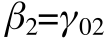
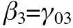
Notice how we would observe variation on the main effect of Y and variation on the intercept. We just replace these with random effects and under the assumptions of random effects, this becomes a stand in for the control parameters.

Where the omegas are the random effects. Random effects in multilevel models do assume them to be normally distributed - that A and B are normally distributed. Finding variation in omega1 takes the place of B. Finding variation in omega0 takes the place of A (and B to some extent due to the scaling issues mentioned above).
As mentioned before, the random effects approach assumes that A & B vary across time series but not within time series. If A & B vary within time series too then those variations come out as error if we are only using random effects to account for A & B. So, once we observe random effects, it makes sense to add possible control parameters for level 1 or level 2 and the control parameter should force the relevant level 2 random effect to zero.
Let's make Change in the outcome. For this example, my variable is Y, I have multiple time series that are separated by an ID variable called ID. We need to first split the file so that the lead variable does not cross different time series.
Now, I am going to run the analysis using the Mixed Command. In this first case, I will assume A and B are unknown, but using random effects to account for them.
Now adding in A and B, but where we still keep the random effects to see if something remains.
Bryk and Raudenbush pointed out that multilevel models are analogous to running a regression within individuals (one for each time series), saving out the regression coefficients and then comparing the coefficients across individuals. They call the equation within cases the Level 1 Equation and the Equations comparing coefficients between cases as the Level 2 Equations. The actual equation tested under Maximum Likelihood is the nested (or mixed) equation where the coefficients in level 1 are replaced with the equations in Level 2. Also, maximum likelihood estimation is an asymptotic estimation procedure. So, estimates are always population based calculation. Thus, error terms are represented by error variances (and a model might have a couple of them known as random effects).
So, let's say that the level 1 equation is the cusp catastrophe regression equation earlier. The only change I will make is to switch to greek symbols because of ML being an asymptotic procedure (greek for population, old statistical norm).
And let's say that the level two equations just had intercepts (no predictors, no residuals). This is like saying that everyone has the identical level 1 equation:
The nested equation (actual equation tested) just combines the level 1 and level 2 equations:
Scaling and Expanding the Equation Form
Now the equation above is imperfect. It is based on the
topological formulation of the cusp catastrophe. It is
mathematically correct, based on a scale free nature. However,
multilevel modeling (and regression too, so what I am about to say
would also apply to the earlier parts) generates partial derivative
relationships. The moment we add interactions and polynomials,
many of the terms lose their scale free nature. To see the issue,
let's go to a much simpler regression circumstance:Y=b0 + b1X + b2Z + b3XZ + e
Here, X and Z interact to predict Y. This interaction is represented by a product term. The key question relevant to our discussion: How do we interpret the main effects of b1 and b2 respectively? B1 is conditional on the scaling of Z and b2 is conditional on the scaling of X. That is, both are interpreted when the other variable from the interaction is zero. Change the scaling of Z and b1 changes - this is the loss of the scale free nature. So, there is some value of Z where b1 would be zero and thus the equation would be correct to actually drop b1 from the equation entirely. At any other value of Z, b1 would be non-zero and by leaving it out we bias the other estimates. There is an exception to this having to do with nested data structures and these nestings often exist in multilevel models, but that is not what is going on here.
Returning to our Regression based Cusp Catastrophe, now including all the implied lower order terms, we have
By leaving out these additional terms, we are assuming they are zero and the extent to which they are not will lead to incorrect solutions.
This leads to two directions to resolve the scaling issue:
- The literature suggested solution is to put all the variables (Y, A, & B) into some form of standardized metric. This logic is based on the notion that centering the zero values will provide the proper estimates. Personally, I believe this is flawed. This should only work to the extent to which the zero values are at the set point and the cusp catastrophe has multiple set points that can even change location. So, it is unlikely to work across the board especially when you are dealing with multiple time points.
- Expand the multilevel model to include all the lower order terms. I am a big fan of this, because it does not put the honess of scaling on the user and will always give proper estimates for the key terms. Some of these actually have topological meaning while others do not. This actually is a problem because it means we are mixing alternate topological interpretations with scaling issues. So, I highly recommend graphing results to see what is going on, much like the graphs I made above. Note that fully expanding the equations does not mean that one can ignore scaling. In fact, the exact opposite is true. The polynomials can all be highly correlated and Maximum Likelihood can actually fail to get proper estimates. However, the solution is just to follow the common rules for scaling in multilevel models (grand centering and group centering).
Random Effects in the Cusp
Butner, et. al. (In Press) conducted the cusp catastrophe model with implied, but unknown control parameters. The way we did this was by careful use of random effects. To understand how this works, we need to talk about the nature of a random effect, also known as a variance component. Let's assume, for the moment, that A and B vary across individuals, but not within individuals. Recall the common assumption that A & B are varying independently from the rest of the variables changing through time. So, we can argue that there is a distribution of values of A and B across individuals. Now imagine that we never measured A and B. Here would be the same equation without A and B, but where I add question marks instead of the A & B. These question marks are varying contributions. Note that the main effect of A & B collapse because we would just see variation there.Notice how we would observe variation on the main effect of Y and variation on the intercept. We just replace these with random effects and under the assumptions of random effects, this becomes a stand in for the control parameters.
Where the omegas are the random effects. Random effects in multilevel models do assume them to be normally distributed - that A and B are normally distributed. Finding variation in omega1 takes the place of B. Finding variation in omega0 takes the place of A (and B to some extent due to the scaling issues mentioned above).
As mentioned before, the random effects approach assumes that A & B vary across time series but not within time series. If A & B vary within time series too then those variations come out as error if we are only using random effects to account for A & B. So, once we observe random effects, it makes sense to add possible control parameters for level 1 or level 2 and the control parameter should force the relevant level 2 random effect to zero.
Code in SPSS
I am going to work in SPSS Mixed to make this work. We can actually use any multilevel modeling program (HLM, Proc Mixed, MLWin, R, etc.). I am assuming that the file is constructed as a long file (HLM would call this a level 1 file; each line is one instance from an individual). First things first, we need an estimate for the derivative. Now, I have always displayed these as derivatives, but the logic of catastrophe models does not require true derivatives. That is, we can use discrete change instead. So, one option is to create an estimate of the derivative using techniques like the Local Linear Approximation or the GOLD method. Alternatively, we can use discrete change. That is what I will do today. This choice has lots to do with the philosophy of time and its relation to the phenomena of interest. More on this another time (a paper unto itself).Let's make Change in the outcome. For this example, my variable is Y, I have multiple time series that are separated by an ID variable called ID. We need to first split the file so that the lead variable does not cross different time series.
| split file by ID. create Y_lead = LEAD(y 1). split file off. compute y_change = Y_lead - y. execute. |
Now, I am going to run the analysis using the Mixed Command. In this first case, I will assume A and B are unknown, but using random effects to account for them.
| Mixed y_change with y /fixed=y y*y y*y*y |SSTYPE(3) /method=reml /print=solution testcov /random = intercept y |subject(id) covtype(vc). |
Now adding in A and B, but where we still keep the random effects to see if something remains.
| Mixed y_change with y A B /fixed=y y*y y*y*y A B y*B|SSTYPE(3) /method=reml /print=solution testcov /random = intercept y |subject(id) covtype(vc). |